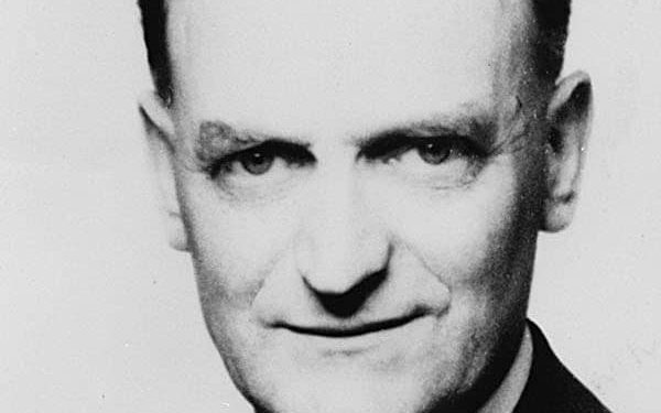
An economic concept which served as the linchpin for monetary and fiscal policy across the world is the Phillips Curve. Developed by the New Zealand economist A.W.H. Phillips, it puts forward an inverse relationship between inflation and unemployment.
Phillips, while he was an economics professor at London School of Economics and Political Science in 1958, tracked wages and unemployment levels in Great Britain from 1861 to 1957 and found that wages rose more rapidly when unemployment rate was low. Contrastingly, when the labour market is tight, there is a greater upward pressure on wages, and through labour costs, on prices.
Source – Wikipedia
Phillips theorized that at a lower unemployment rate, firms must raise wages to attract scarce labour. The total money in circulation rises, resulting in a boost in spending and inevitably increasing inflation. The opposite happens when unemployment rises, wages fall and consequently inflation falls.
Economists soon started estimating the Phillips Curve for most developed countries. The close alignment between the estimated curve and available data encouraged many economists, following the lead of Nobel Laureates Paul Samuelson and Robert Solow, to hail the Curve as a menu for policy options. Governments and central banks worldwide began tolerating higher inflation when they were spending money on job creation.
Source – Bureau of Labour Statistics, U.S.A.
At the height of Phillips Curve’s popularity as a policy guide, Nobel Laureates Edmund Phelps and Milton Friedman independently challenged its theoretical and conceptual underpinnings. They opined that – rational, well informed employers and workers would pay attention only to real wages: the inflation-adjusted purchasing power of money wages.
In their opinion, real wages would adjust to make the supply of labour equal to the demand for labour, and the level of unemployment rate would be uniquely associated with that real wage i.e., the natural rate of unemployment.
Both Phelps and Friedman argued that a government could not permanently trade higher inflation for lower unemployment. Imagine that unemployment is at the natural rate and the real wage is constant: workers who expect a given rate of price inflation demand that their wages increase at the same rate to prevent a fall in their purchasing power.
Now, imagine that governments and central banks use expansionary fiscal or monetary policy in an attempt to lower unemployment below its natural rate. The resulting increase in demand allows firms to raise their prices faster than workers had anticipated. With higher revenues, firms are willing to employ more workers at the old wage rates and even to raise those rates to a particular level. For a short time, workers suffer from what is called money illusion: they see that their money wages have risen and willingly supply more labour. Thus, the unemployment rate falls.
They do not realize that their purchasing power has fallen because prices have risen more rapidly than they expected. But, over time, as workers come to anticipate higher rates of price inflation, they supply less labour and demand increases in wages that keep up with inflation. The unemployment rate returns to the natural rate and the real wage is restored to the old level. But the price inflation and wage inflation brought on by expansionary policies persist at the new, higher rates.
Phelps’s and Friedman’s analyses provided a distinction between the “long-run” and “short-run” Phillips curves. During the 1960s, the average rate of inflation remained fairly constant, resulting in an inverse relation between inflation and unemployment. But if the policymakers persistently try to push unemployment below the natural rate, the average rate of inflation will change.
After a certain period of adjustment, unemployment will return to the natural rate. This implies that once workers’ expectations of price inflation have had time to adjust, the natural rate of unemployment is compatible with any rate of inflation.
Source – Federal Reserve Bank of St. Louis
The long-run and short-run dimensions can be combined to form a single “expectations-augmented” Phillips curve. The faster the workers’ expectations of price inflation adapt to changes in the actual rate of inflation, the faster unemployment will return to the natural rate, and the less effective governments and central banks will be in reducing unemployment through monetary and fiscal policies.
The 1970s validated Friedman’s and Phelps’s fundamental point. Contrary to the original Phillips curve, when the average inflation rate in the U.S.A. rose from about 2.5 percent in the 1960s to about 7 percent in the 1970s, the unemployment rate, instead of falling, rose from 4 percent to above 6 percent. This phenomenon came to be known as stagflation, which occurs when an economy experiences stagnant economic growth, high unemployment and high price inflation, and directly contradicted the Phillips curve.
Most economists now accept a central credo of both Phelps’s and Friedman’s analyses: there is some rate of unemployment that, if maintained, would be compatible with a stable rate of inflation. Nowadays, the expectations-augmented Phillips curve is a fundamental element of almost every macroeconomic forecasting model used by governments, central banks and businesses. It is accepted and recognised by most otherwise diverse schools of macroeconomic thought.
Recently, however, researchers from Columbia University and the University of Chicago have questioned the robustness of the Phillips curve in terms of price inflation. Studying data from 1988-2018, they conclude that the Phillips curve seems to be hibernating in U.S.A., but can return with inflationary pressures rising in the face of an overheating labour market.
Nevertheless, at least part of Phillips’ troublesome trade-off lives on. When faster economic growth and full employment return, you can bet inflation will be along to spoil the party!
Written by- Kanishq Chhabra
Edited by- Nanditha Menon
The post The Controversial Curve appeared first on The Economic Transcript.


